My current project is an automated Lego sorting machine. I’ve seen a few other blogs showing off their Lego sorters. They’re super cool! But they usually show off the completed final result and skip all the interesting learning that happened along the way. This series is going to be the build log of the process of designing, building and programming this thing.
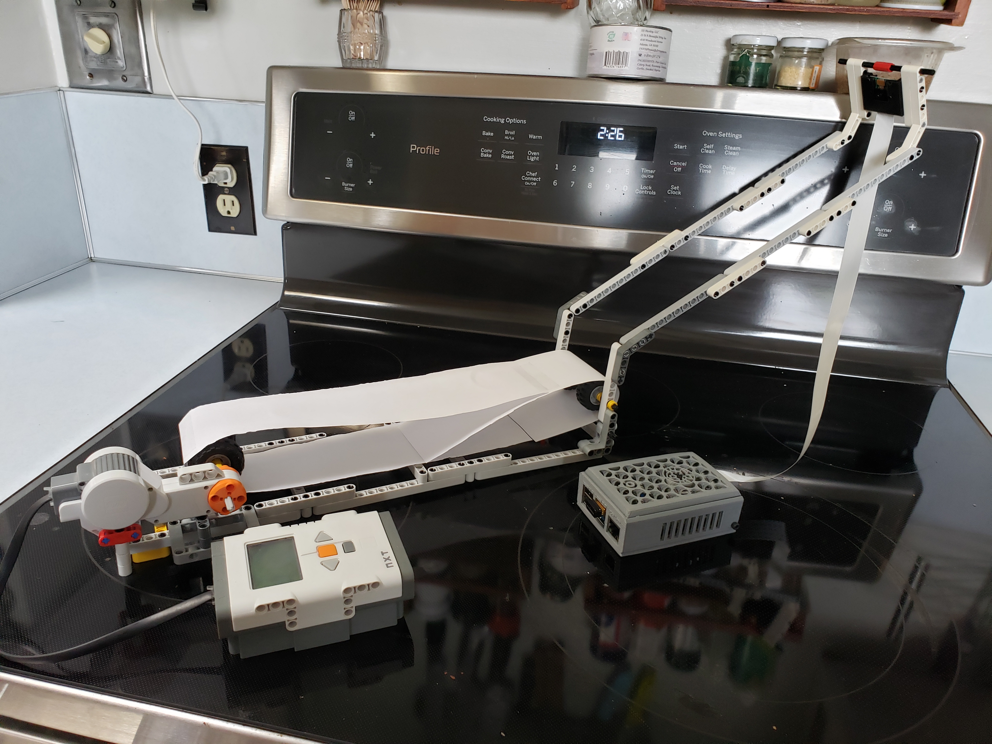
So far, the sorter does… well, nothing. But that’s getting a bit ahead of the story. For now, here’s a pick of the current “sorter”. It doesn’t look like much yet. In fact, it looks pretty… uh, janky.
How This Started
The way some people are “Disney People”, my family are “Lego People”. We scan the monthly Lego advert and plan the sets we just have to have; We’ve been to Legoland multiple times; We own shelving units that are dedicated purely to Lego; We have built an 18"x18"x24" “end table” that is solid bricks.
Suffice to say, we like playing with Lego bricks.
But as anyone who has ever played with Lego knows, when it comes time to put them away, you can either throw them all in a pile or spend twice as much time sorting as you did building.
After your Lego collection reaches a certain size, sorting becomes a necessity.
Automated Lego Sorting
There have been multiple Lego sorter projects using computer vision and neural networks to recognize and sort Lego. This one is mine.
Neural Networks
Heavily inspired by Daniel West’s project, I decided to start off by setting up a Neural Network (NN) to identify Lego brick. I haven’t touched neural networks or really AI of any sort since my college days… fifteen years ago, so I’m starting basically fresh.
The first thing I learned is that almost no one writes their own NN from scratch anymore, instead making use of one of many high-quality libraries available, such as PyTorch, TensorFlow, Keras or Scikit-Learn.
While there are many things to recommend each of these libraries, I decided to go with Keras, largely due to its simplified interface. I’m flying by the seat of my pants here, might as well make it easy on myself.
Getting Data
Anyone who works with Neural Networks can tell you that the first hurdle to getting a network running is getting clean and labelled data to train your model on. Waiting until my sorter was fully built and functioning was a non-starter for me. I want to start working on the brains in parallel with my crummy Lego build efforts. But in the absence of captured data, I need to create some simulated data quickly.
Enter LDraw.
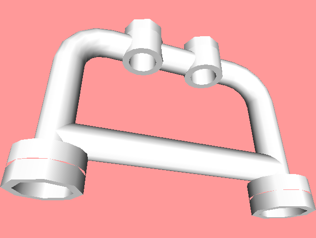
LDraw is a CAD standard for Lego bricks. Every Lego brick so far in existence (well, mostly) has an LDraw file. I use these to generate simulated images of Lego bricks. Like this:

Look at all that detail!
…in fact, probably too much detail. My real-world Lego images won’t be nearly this clean. But that’s OK! Right now, I just want to sanity check my model and see if I can make a network that recognizes a handful of Lego brick.
LDView
Ok, I cheated a little bit right there. See, LDraw files are great - but they don’t do anything by themselves. You need a viewer to interact with them. There are a number of options, but I chose LDView because it a) runs on Linux and b) provides a comprehensive command-line interface. I need the latter so that I could script up generating hundreds of images per part.
LDView <filename>
 -DefaultColor3=0x00FF00 \
 -BackgroundColor3=0xFF9999 \
 -DefaultLatLong=0,0 \
 -DefaultZoom=1 \
 -WindowHeight=240 \
 -WindowWidth=320 \
 -SaveSnapshot=<output_filename>.png"
Generator
I wrote a quick Ruby script that iterated over piece types (I chose 100 random piece IDs from the LDraw set), piece colors (DefaultColor3) and rotations (DefaultLatLong) and then invoked LDView with the appropriate command line arguments. Each image took around 2 seconds to generate and I generated 150 random images per part. To speed up calendar performance, I created a Queue and had multiple threads pull work off of it to perform. For each part, I generated 150 “jobs” and pushed them all onto the Queue. Each Thread then popped the next item off the queue and generated an image of the specified part.
Why 150 parts? It seemed like a high enough number to get results, while small enough to generate in a reasonable amount of time.
Anyway, after generating, the script stored the generated images in directories which shared a name with the original Lego ID number. e.g. if the Lego ID was 4083 (the piece above), then all the generated images of that piece would be in a directory named 4083. This will help us later on with Keras.
Network Modelling
Now we have some data! It probably won’t translate well into real-world performance (lighting differences, for instance, can make a huge difference!) but it’s enough to get started with and see if we can train a model to recognize our simulated bricks.
The type of Neural Network we’re using is called a Convolutional Neural Network. This type of network is well suited for computer vision applications.
There are a lot of tutorials on setting up Keras, so I’m going to skip that part and get right to the good stuff. Modelling with it.
For a CNN we need to do a few things. Normalize the data; Define the Network itself; and then generate our predictions. Keras makes all of this easy.
Keras represents stages in your data pipeline as “layers”. You can define Input layers that do things like scale or normalize your data, network layers that make up the “smarts” of your model, and output layers that provide your final predictions. Let’s take a look at what I did.
0. Define your Model’s Input and Output
This is where we tell Keras what we want the “shape” of our input and output data to be. Output is a list of probabilities, between 0-1 that indicates how “confident” the network is that a given image falls into a given class.
For instance, if we had 5 types of pieces that we recognized, our output would be an array of 5 values between 0 and 1. In a well trained network, we would expect the highest value to correspond to the actual piece.
The input represents the shape of the Image data we’re passing in. For my training data, the shape is 320x240x3 (320x240 pixels, each containing 3 RGB values for color).
The input, we describe directly. The output is taken from the shape of our final layer’s output.
 inputs = keras.Input(shape=(320, 240, 3))
 layers = build_model(inputs)
 outputs = output_layers(num_classes, layers)
1. Normalize the Data
Neural networks have an easier time when the data is formatted as floating point values between 0 and 1. For our use case, that means scaling all of the RGB color values from 0-255 to 0-1. For me, that just meant a single Rescaling layer:
layers = Rescaling(scale = 1.0/255)(inputs)2. Define the Convolutional Layers
This is an area that I’m still learning heavily. I did this bit by luck and some educated guesses. I have almost certainly done this “horribly wrong” and will need to tweak this once I start getting real data. But…
A Convolutional layer takes a kernel (here a 3x3 set of pixels) and sums their values together to create a single “pixel” value for the next layer of the network. This has the effect of making features stand out more effectively in the next layer of the network.
In between each Convolutional layer is a pooling layer. Pooling layers basically take a set of pixels (in this case a 3x3 square) and map to a single value in the next layer. As the features become more defined, we can throw away some of the data to have a smaller representation. This allows us to shrink the size of our data so that later training isn’t as computationally expensive.
cl = Conv2D(filters=32, kernel_size=(3,3), activation="relu")(layers)
cl = MaxPooling2D(pool_size=(3, 3))(cl)
cl = Conv2D(filters=32, kernel_size=(3,3), activation="relu")(cl)
cl = MaxPooling2D(pool_size=(3, 3))(cl)
cl = Conv2D(filters=32, kernel_size=(3,3), activation="relu")(cl)
I’m doing three layers of convolution with pooling in between. Why?
I say, why not?
3. Generate Output
This is the “smart” bits of the network, where we adjust weights and teach the network to generate the output we want. It’s also the final part of the network that ultimately spits out the class of object it thinks we have.
ol = Dropout(0.25)(layers)
ol = Flatten()(ol)
ol = Dense(units=64, activation='relu')(ol)
ol = Dense(units=num_classes, activation='softmax')(ol)
Here we first have a Dropout layer, where we simply drop some percentage of the output from the previous layer. This helps us avoid overfitting our model.
Next we take our 2-D data and Flatten it to a 1-D list of values. This is easier for our NN to work with.
Finally, our two Dense layers are where the real magic happens. In a Dense layer, each input node is connected to each output node, but with differing weights. The first Dense layer here has N input nodes (where N is the number of values spat out by Flatten) and 64 output nodes. Those 64 output nodes are then connected to the next Dense network which has num_classes output nodes. Where (in this case) num_classes is the number of Lego parts we know about and are training the model on.
Training
Phew!
After that set up, we’re finally ready to run the model on our generated Lego images. We want to split our data into training and validation data to help guide the model fitting process. If we structured our input like above, with each image set in its own labelled directory, Keras will automatically create the appropriate number of data classes for us. (I told you that would come in handy!)
# Import dataset
training = keras.preprocessing.image_dataset_from_directory(
    '/home/lucas/Projects/bricksorter/training_data',
    validation_split=0.2,
    subset="training",
    seed=1337,
    batch_size=64, image_size=(320, 240))

validation = keras.preprocessing.image_dataset_from_directory(
    '/home/lucas/Projects/bricksorter/training_data',
    validation_split=0.2,
    subset="validation",
    seed=1337,
    batch_size=64, image_size=(320, 240))

num_classes = len(training) # Number of directories in training data

# Create our model layers
...

# Create the Model object
model = keras.Model(inputs, outputs)

# Compile the model
model.compile(optimizer='rmsprop', loss='sparse_categorical_crossentropy')

# Fit the model
model.fit(training, validation_data=validation, epochs=10, callbacks=callbacks)
So… How’d it Work?
Great. Feeding newly generated sim images that the network hadn’t seen before, I got highly accurate results. Almost every piece I tried I got an accurate prediction for. Some orientations were harder to predict of course (lots of pieces look the same, edge on), but I am very encouraged by this!
Next Steps
Now that I have a prototype CNN to test against… it’s time to start capturing some real-world image data to start training and testing against.
…Which brings us back to that conveyer-belt Lego prototype. Next blog post I’ll talk about how that works and the software we need for it.
